ISSUE 5: When is lead, lag, and why is yesterday perfectly correlated with today?
You have to be careful when working with lagged components of a time series. Note that lag(x,1) is a FORWARD shift and lag(x,-1) is a BACKWARD shift. Try a small example:
x=ts(1:5)
cbind(x,lag(x,1),lag(x,-1))

Time Series:
Start = 0
End = 6
Frequency = 1
  x lag(x, 1) lag(x, -1)
0 NA         1         NA
1  1         2         NA
2  2         3          1
3  3         4          2 <-- here, x is 3, lag(x,1) is 4, lag(x,-1) is 2
4  4         5          3
5  5        NA          4
6 NA        NA          5
Note that the default of the command lag(x) is lag(x,1). So, in R, if you have a series x(t), then
y(t) = lag{x(t)} = x(t+1), and NOT x(t-1).
This seems awkward, and it's not typical of other programs. But, that's the way Splus does it, so why not R? As long as you know the convention, you'll be ok ...
... well, then I started wondering how this plays out in other things. So, I started playing around with some commands. In what you'll see next, I'm using two simultaneously measured series presented in the text called soi and rec... it doesn't matter what they are for this demonstration. First, I entered the command
acf(cbind(soi, rec))
and I got:
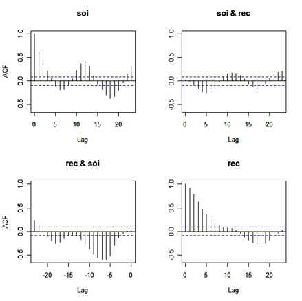 |
Before you scroll down, try to figure out what the graphs are giving you (in particular, the off-diagonal plots ... and yes they're CCFs, but what's the lead-lag relationship in each plot???) ...
.
.
.
.
.
.
.
... here you go:
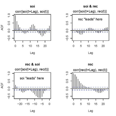 |
The jpg is messy, but you'll get the point... the writing is mine. When you see something like 'rec "leads" here', it means rec comes in time before soi, and so on. Anyway, to be consistent, shouldn't the graph in the 2nd row, 1st column be corr{rec(t+Lag}, soi(t)} for positive values of Lag ... or ... shouldn't the title be soi & rec?? oops.
Now, try this
ccf(soi,rec)
and you get
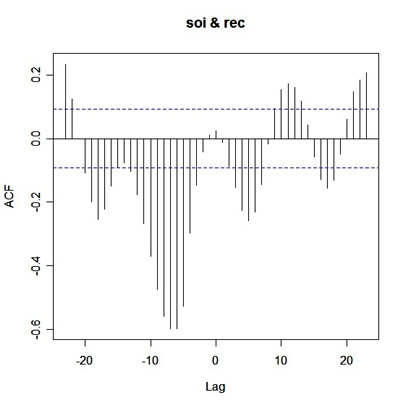 |
What you're seeing is corr{soi(t+Lag), rec(t)} versus Lag. So on the positive side of Lag, rec leads, and on the negative side of Lag, soi leads.
We're not done with this yet. If you want to do a regression of x on lag(x,-1), for example, you have to "tie" them together first. Here's an example.
x = arima.sim(list(order=c(1,0,0), ar=.9), n=20)  # 20 obs from an AR(1)
xb1 = lag(x,-1)
## you wouldn't regress x on lag(x,1) because that would be progress :)

##-- WRONG:
cor(x,xb1)  # correlation
  [1] 1     ... is one?
lm(x~xb1)   # regression
 Coefficients:
 (Intercept)          xb1
   6.112e-17    1.000e+00
do it the WRONG way and you'll think x(t)=x(t-1)


##-- RIGHT:
y=cbind(x,xb1)   # tie them together first
lm(y[,1]~y[,2])  # regression
 Coefficients:
 (Intercept)       y[, 2]
      0.5022       0.7315

##-- OR:
y=ts.intersect(x,xb1)  # tie them together first this way
lm(y[,1]~y[,2])  # regression
 Coefficients:
 (Intercept)       y[, 2]
      0.5022       0.7315
cor(y[,1],y[,2]) # correlation
 [1] 0.842086

By the way, (Intercept) is used correctly here.
R does warn you about this (type ?lm and scroll down to "Using time series"), so consider this a heads-up, rather than an issue. See our little tutorial for more info on this.
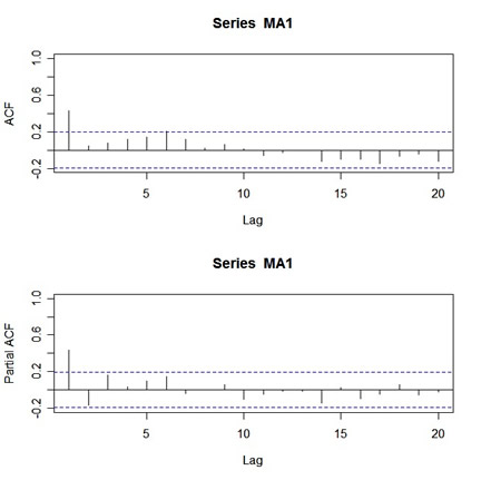
ISSUE 6: Why do you want to see the zero lag value of the ACF, and what's this mess?
When you're trying to fit an ARMA model to data, one of the first things you do is look at the ACF and PACF of the data. Let's try this for a simulated MA(1) process. Here's how:
MA1=arima.sim(list(order=c(0,0,1), ma=.5), n=100)and here's the output:
par(mfcol=c(2,1))
acf(MA1,20)
pacf(MA1,20)
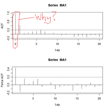 |
What's wrong with this picture? First, the two graphs are on different scales. The ACF axis goes from -.2 to 1, whereas the PACF axis goes from -.2 to .4. Also, the lag axis on the ACF plot starts at 0 (the 0 lag ACF is always 1 so you have to ignore it or put your thumb over it), whereas the lag axis on the PACF plot starts at 1.
So, instead of getting a nice picture by default, you get a messy picture. Ok, the remedy is as follows:
par(mfrow=c(2,1))and here's the output:
acf(MA1,20,xlim=c(1,20)) # set the x-axis limits to start at 1 then
# look at the graph and note the y-axis limits
pacf(MA1,20,ylim=c(-.2,1)) # then use those limits here
 |
Looks nice, but who wants to get carpal tunnel syndrome sooner than necessary? Not me. So I wrote an R function called acf2 that will do everything at once and save you some time and typing. You can get acf2 on the web page for the text under R CODE (Ch 1-5) - use the blue bar on top of this page to get there.
Comentarios
Publicar un comentario